The offsets

The mode decides the rows. The offsets decide which slice of
time the task reads, and which part of the result it is willing to write.

There are three. Two of them look identical from the outside: both delay your newest
value, and setting either to zero leaves the same wrong number behind, so they are
best read together:

Setting	Moves	Effect
Realtime offset	Where the window ends	Stops short of now, so late data can land. Adds lag.
Start offset	Where reading begins	Reads earlier than the window, as context. No lag.
Output hold-back	Where writing ends	Withholds the newest results until their window closes. Adds lag.

One window is read, and a smaller one is written

Every setting above is a gap between two edges: everything the task reads, and the
part of it the task is willing to write.

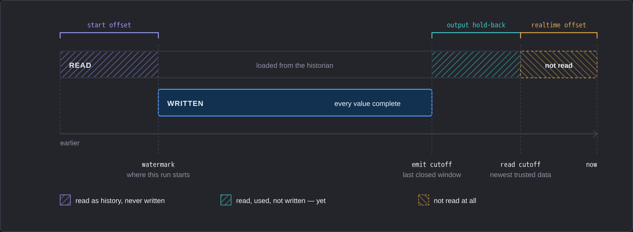
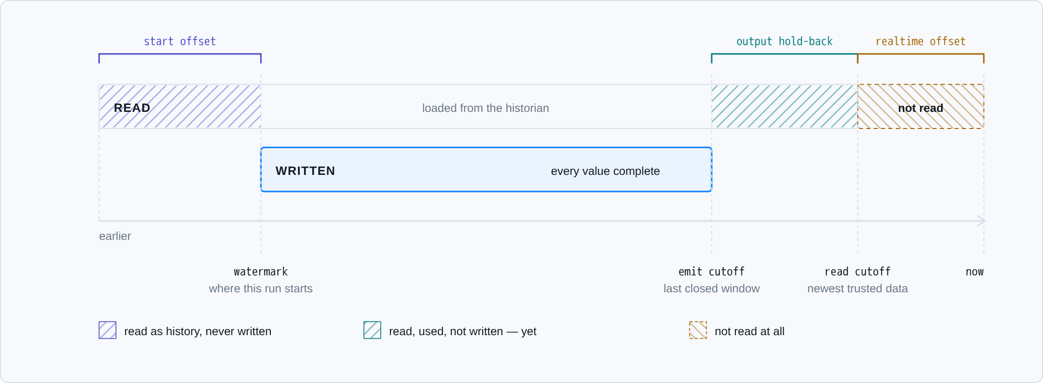
The one thing to take from the picture: the hold-back band is inside the read bar,
and the realtime band is outside it. Hold-back data is loaded and used: it is the
context that makes the values before it correct: it just is not written yet.
Realtime-offset data is never fetched at all, because it may not have arrived.

The same explanation lives in the product

The Time Alignment tab has an Offsets button beside the fields. It opens this
figure, the decision below, and the quick reference, so you do not have to come back
here mid-configuration.

Which one does my script need?

The start offset and the hold-back are two answers to one question, not two knobs
to tune. One question decides between them, and it is a question your calculation
already answers:

Does the value stamped at time T describe the period before T, or after it?

	It describes time before T	It describes time after T
Why	The value summarises the period leading up to its own timestamp, so it cannot be computed until that history exists.	The value summarises the period that starts at its own timestamp, so it is not finished until that period is over.
It needs	History	The future
Start offset	= your window	0
Output hold-back	0	= your window
Examples	rolling(), ewm(), diff(), cumsum(), resample('1h', label='right')	resample('1h') with no label: the pandas default

At most one of the two is ever set

They are two answers to one question. Setting the wrong one is not merely useless: a
hold-back on a backward-looking script buys a full window of latency for values
that were never incomplete, and a start offset on a forward-looking one buys extra
reads that do nothing.

Note which arm the pandas default falls on. resample('1h') with no label argument
is the after-T family, so a plain resample wants hold-back and no start offset:
the opposite of what the worked example below needs.

The worked example

Suppose your calculation resamples a channel to hourly means:

y1 = x1.resample('1h', label='right').mean()

This is a Timeseries Dataframe
calculation: x1 arrives as a timestamp-indexed DataFrame, so resample has something to
work with.

Note label='right'. It is doing the work here: it stamps each bin at the end of
its interval, so the mean of 09:00–10:00 is written at 10:00: a value describing the
hour before its own timestamp. That is the left-hand arm: it wants a start offset,
and hold-back stays at 0.

pandas labels bins on the LEFT by default

x1.resample('1h').mean(), with no label, stamps the mean of 09:00–10:00 at
09:00, not 10:00. The value then describes the hour after its timestamp, which
puts it on the right-hand arm: it wants hold-back, and no start offset.

label moves only the label, never which readings go in the bin. closed still
defaults to 'left', so a bin stamped 03:00 covers [02:00, 03:00): a reading exactly
at 03:00 belongs to the next bin. With readings 02:00=1, 02:30=2 and 03:00=99, the
value stamped 03:00 is 1.5, not 34.

Now run the label='right' version over a window starting at data start:

With start offset 0, the task begins reading at data start. The first complete
hour of data ends one hour later, so the first output row is at data start + 1h.
You wanted a value at data start, and there is a one-hour hole at the front of every
run.

With start offset = 1h, the task begins reading one hour before data start. By
the time it reaches data start it already has a full hour behind it, so it can emit a
value stamped data start. The rows computed from that prefetched hour are stamped
before the window start, so they are discarded: they existed only to prime the
calculation.

The newest bin waits for its interval to close

A right-labelled resample writes one fewer bin per run than you might count: the bin
covering the period the run stopped inside is not written yet. It appears on the next
run, once that interval has closed and the value is complete.

If you are comparing output from before and after an upgrade, that missing trailing bin
is the difference: the value that used to appear there was computed from a partial
interval.

Start offset; read earlier than you write

Start offset reads earlier than the window start. The extra rows are context: they
are used, and then discarded rather than written. Nothing before the window start
ends up in your output, so this costs reads and never costs latency.

Match it to your longest window

Set the start offset to at least the longest window your calculation looks back over.
A one-hour resample needs an hour. A 24-hour rolling average needs 24 hours. Less than
that and the leading rows are computed from partial data: which is worse than the gap,
because the numbers look plausible and are wrong.

This applies to anything that reaches backwards: label='right' resamples, rolling,
ewm, diff against a previous value, cumulative totals, and any filter with a
warm-up. It does not apply to a default left-labelled resample: that one wants the
hold-back instead.

Output hold-back: do not write an unfinished window

The problem it solves

A one-hour average asked for 05:00–06:00 at 05:30 can only see thirty minutes. It
returns the mean of those thirty minutes: a real number, in range, plausible, and
wrong.

And it is permanent. This is the part worth understanding, because the obvious
assumption is the opposite. You might expect the next run to correct it once the hour
completes. It does recompute the window correctly, and then discards its own
answer, because that timestamp now sits below the new run's output floor. Today's
partial trailing value is not provisional. It is final, and nothing will revisit it.

So a forward-looking calculation with no hold-back writes exactly one wrong value per
run, forever, at the newest end of its output.

How it works

Hold-back does not stop the task reading the newest data. That data is read and
used as context: it contributes to windows that are complete. What hold-back stops
is emitting results in the trailing region, until the window covering them has
closed.

The diagram beside the fields on the tab shows this directly, and redraws itself as you
change the values:

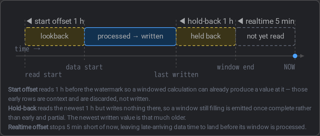
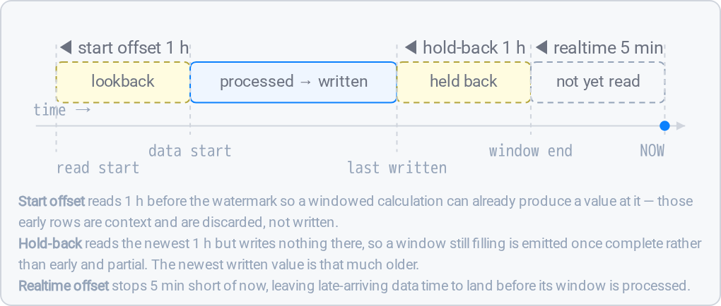
Two dashed bands flank the solid one, and both dashed bands mean the same thing:
read, but not written:

Band	Meaning
lookback	Read as context. Rows here are stamped before the window start and discarded.
processed → written	Read, computed, and written.
held back	Read as context. Results here are withheld until their window closes.
not yet read	Outside the window entirely: the realtime offset's grace period.

last written is the tick hold-back moves. Set hold-back and it slides left, away from
the window end; set it to zero and the two coincide.

The cost, stated precisely

Exactly one window of lag on the newest value. No more, and it does not accumulate:

At 05:30, with a plain resample('1h')	Newest value emitted
Hold-back off	05:00, computed from 30 minutes of data, never corrected
Hold-back = 1h	04:00, computed from the full hour

Read that table carefully, because it is easy to see it as a downgrade. It is not a
delay in getting correct data: the correct 05:00 value did not exist at 05:30 and
could not have. What hold-back removes is a wrong early value. The newest stamp
goes from 0–1 windows old and partial, to 1–2 windows old and complete.

When to use it

Set it, to your window, when the value stamped at T describes the period after T,
and especially when the output feeds anything that treats a written value as final:
a report, a billing figure, a KPI table, an archive. Those are the cases where one
wrong newest row is worst, because nothing downstream expects to re-read it.

Leave it at zero when:

• Your calculation is backward-looking. Use the start offset instead; a hold-back
  here is pure latency for values that were already complete.
• The calculation is point-by-point: a ratio, a conversion, a threshold. Every row
  is complete the moment it exists, so there is no unfinished window to hold.
• The output drives a live display where freshness matters more than the newest
  point being final, and a slightly wrong latest value is acceptable because a human is
  watching it move.
• The mode is Snapshot. It emits one value at the run time by definition, so there
  is no trailing window; the setting is ignored and the tab says so.

The realtime offset is a different question entirely

The realtime offset sits at the same edge of the window as the hold-back, which is why
the two get confused. It is answering something else.

	Realtime offset	Output hold-back
The question	Has the data arrived?	Is the window complete?
What is wrong	The events exist, a sensor recorded them, but they have not reached the historian. A driver reconnected; a buffer has not flushed. A reading stamped 10:03 turns up at 10:06.	The events do not exist yet, because the time they would cover has not happened. An hourly average of 05:00–06:00 cannot be computed at 05:30 however perfect your network is.
Kind of problem	Delivery. It lives in your plumbing.	Arithmetic. It lives in your script.
How you pick it	You measure it: a little more than the worst lateness you actually see.	You read it off the script: it is the window length, and nothing to do with your infrastructure.
What it changes	The window itself. Less is read.	Only what is written. The data is still read and used.

Think of a monthly sales report. You do not publish January's total on the 20th:
January is not over. That is hold-back. You do not publish it on 1 February either,
because some receipts are still in the post. That is the realtime offset. Two
waits, two reasons, and a careful accountant wants both.

And here is why nobody can keep them apart: set either to zero and the symptom is
identical: a wrong value at the trailing edge that is never corrected. The symptom
is the same; the cause is not.

They stack. The newest value a task emits is roughly
now − realtime offset − output hold-back. Setting both to an hour puts your newest
value two hours behind: which may be correct, but should be a decision rather than a
surprise.

If Stream sees both a start offset and a hold-back set on one task, it says so beside
the fields. It is a hint rather than an error: nothing breaks, because the service uses
the larger of the two.

Does any of this apply to my task?

What makes a task windowed is the variable-passing mode, not what it writes to. A
table task in Timeseries Dataframe mode sees a whole page at once, so one of its
columns can be a rolling mean, and it needs the hold-back exactly as a channel
calculation does.

Task shape	Windowed?	Needs hold-back?
Table or JSON mapping, no calculation	No	No. Use the realtime offset if you are waiting on late data.
Calculation in per-row (scalar) mode	No	No: each row is computed from that row alone.
Calculation in Timeseries Dataframe mode	Yes	Yes, if the value describes the time after its timestamp.
Channel calculation (writes back to tags)	Usually	Yes, if it is windowed.

Stream applies this for you: where the hold-back can do nothing, the field is replaced
by a line saying why, rather than accepting a number and ignoring it.

One difference between output types, because it is observable

On table, JSON and SQL output the hold-back is applied per run; on channel
calculations it is applied per page as well. What you see: on a table task the withheld
rows arrive on the next run rather than later in the same one. For a live task that
is invisible. For a long backfill it means the last window of each run lands on the
following run.

Why isn't it just a switch?

The reasonable version of the question: why not a checkbox that says do not write
incomplete windows, and let Stream work it out?

Because Stream cannot see your window. Your script is arbitrary Python: Stream hands
it dataframes and gets back timestamps and numbers. It never sees '1h', and it never
sees label=. A switch would have to infer completeness, and the inference does not
hold:

• Output spacing is not the window. rolling('24h') on one-minute data emits a
  value every minute from a twenty-four-hour window. Inferring the window from the
  spacing is wrong by a factor of 1440.
• One case is detectable, and is already handled. A value stamped after the
  newest input is provably incomplete, which catches the whole backward-looking family.
  Stream withholds those automatically, with no setting: output never runs past the end
  of the window it was computed from.
• The other case is invisible. Forward-looking, the half-finished value is stamped
  inside the data range and looks exactly like a finished one. Nothing in the output
  distinguishes it, so nothing can catch it.

Which is the real answer to the question: the half a service can see is automatic
already, and the setting exists for the half it cannot. That is also why the two arms
differ. On the backward-looking arm, hold-back 0 is not merely acceptable: it is
exactly right, because that arm is covered without it.

What's Next

With the window settled, see how a long one is read in
pages, or go straight to what each row contains, in
Task Calculation →.

Related

• Time Alignment: the mode these offsets apply to
• How a run is paged: what happens when a window is too large to read at once
• Task Calculation: the windowed calculations these offsets exist for