Task Calculation

The Calculation tab is where a task derives new values from the ones it read. It
appears when you chose Python calculation as the task's transform.

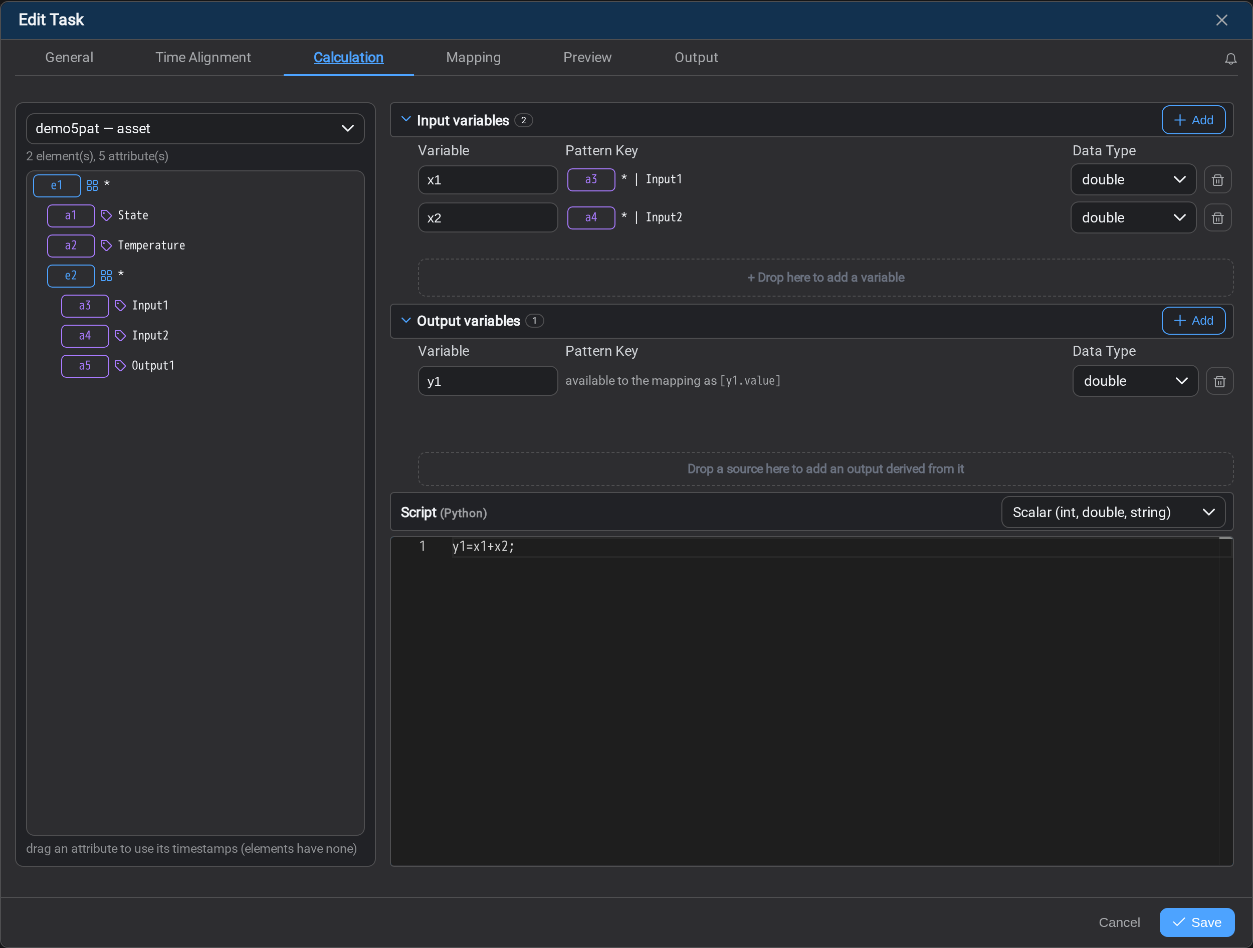
The tab is in three parts, and they read left to right, top to bottom:

1. The source pane on the left: what this task can read
2. Input and output variables on the right: the names your script will use
3. The script underneath: what to compute

The whole arrangement exists to do one thing: let you write a formula once and have it
run against every match the pattern produced.

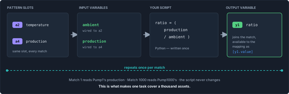
An input variable is a name bound to a pattern slot. The script uses the name; the
slot supplies that match's value. An output variable is a name the script assigns to,
and it joins the match alongside the pattern's own slots: which is how the
mapping can write it out afterwards.

The source pane

The left pane lists what the task's source makes available. For a pattern task,
that is the pattern's tree: its elements and attributes, each with the key you
gave it when you built the pattern.

You do not type these names into the script. You drag them across into the
variable lists, which is how the script gets a stable name to work with.

Input variables

An input variable connects one thing from the source to one name in your script.

Column	What it is
Variable	The name your script will use: x1, inletTemp, whatever you choose
Pattern Key	Which part of the source it reads
Data Type	What to treat the value as

To add one, drag an attribute from the left pane into the drop area, or select
Add and choose. Then rename the variable to something you will recognise in the
script: the defaults are x1, x2 and so on, which work but do not read well in a
formula six months later.

Why the variable points at a key, not a name

This is the part worth understanding, because it is the whole reason one formula can
serve a thousand assets.

The input points at the pattern's key, a3, not at an attribute called
Input1. The pattern already guarantees that every match has something in the a3
position, so on each match a3 resolves to that combination's attribute, whatever
the asset happens to call it.

Take the weather-station example: a pattern pairing a weather station with each pump
beneath it, where a2 is the station's temperature and a4 is the pump's production
rate. You write:

efficiency = production / ambient

with ambient wired to a2 and production wired to a4. On match 1 that reads
pump 1's rate; on match 1000 it reads pump 1000's. The station's temperature comes
along in every match because the pattern paired it there.

One formula. A thousand runs. Nothing to edit when pump 1001 arrives. That is
what you are buying by wiring to keys rather than names.

Data types

Type	Use for
double	Ordinary process measurements: the usual choice
int32, int64	Whole numbers, counters
bool	True/false states
string	Text
enum	A value from a fixed set of states

Pick the type that matches what the attribute actually holds. Stream fills this in
from the pattern where it can, so check it rather than assuming: a value read as
the wrong type is a run that fails on the first asset with real data in it.

Output variables

An output variable is a result your script produces. Give it a name and a data type;
the script assigns to that name.

Underneath each output, the tab tells you how it will be referred to later, for
example available to the mapping as [y1.value]. That is the token you will use
on the Mapping tab to put this result into a column.

For a write-back task there is no Mapping tab: the output goes back into the PI
System, and you point it at the pattern key it should be written to.

You can also drag a source into the lower drop area to create an output derived from
it, which sets up the naming and type for you.

The script

Write plain Python. Read the input variables by name, assign to the output
variables by name.

The example in the screenshot is the whole idea in one line:

y1 = x1 + x2

Two inputs, one output. A real calculation looks the same, just longer:

delta = inletTemp - outletTemp
efficiency = (delta / inletTemp) * 100

Only the declared output variables are kept. Intermediate values like delta above
are fine: they simply are not written anywhere.

The Python that runs it

Stream runs your script on an embedded Python 3.14.6. You do not install it,
configure it, or manage its packages, and there is no environment to keep in step
across servers: the interpreter ships with the service.

Four scientific libraries are preloaded and ready to import:

Library	Version	Good for	Documentation
NumPy	2.5.1	Fast array maths, vectorised arithmetic, linear algebra	numpy.org/doc/stable
SciPy	1.18.0	Signal processing, filtering, curve fitting, statistics, optimisation	docs.scipy.org/doc/scipy
pandas	3.0.3	Time-series handling: resampling, rolling windows, joins	pandas.pydata.org/docs
Polars	1.42.1	The same shape of work as pandas, faster on large DataFrames	docs.pola.rs

pandas is 3.x

Most pandas examples online are written for 1.x or 2.x, and several defaults moved
between then and now. If you copy a recipe and it behaves unexpectedly, check it
against the 3.x documentation before assuming the
data is wrong.

Three more packages come along as pandas' own dependencies. They are importable and
they work, but they are present rather than chosen; treat them as a lower tier
than the four above:

python-dateutil 2.9.0.post0 · six 1.17.0 · tzdata 2026.3

The set is fixed, and the versions do not drift

There is no pip in the bundle and no way for a deployment to add a library. The
runtime is not installed: it is extracted from a single versioned archive that ships
with the service, with every library vendored inside it. Adding one means a new build
of Stream, not a change on your server.

The versions above are pinned exactly, not as ranges, so a redeploy cannot quietly move
you to a different pandas. If you need to cite a source rather than a list of numbers,
the archive names the interpreter version itself:

dependencies/python-3.14.6-embed-amd64.zip

The language itself is documented at
docs.python.org/3, and the
standard library reference covers math,
statistics, datetime and the rest without any import beyond the usual.

pandas is the one most calculations reach for, because Stream can hand your
script a time-indexed DataFrame directly; see the next section.

How your variables reach the script

The Pass / retrieve variables as control beside the Script box decides the shape
your variables arrive in. It is the most consequential setting on this tab, because it
changes what your code can do.

Mode	Each input variable is	Your script runs
Scalar (int, double, string)	one single value	once per row
Timeseries Dataframe	a timestamp-indexed DataFrame of the whole page	once per page

Scalar: one row at a time

The default. Each input holds one number (or string, or boolean): the value for the
row being processed, and each output takes one value back.

y1 = x1 + x2

This is exactly right for unit conversions, ratios, efficiencies, thresholds, and
anything else that depends only on the values in front of it:

delta      = inletTemp - outletTemp
efficiency = (delta / inletTemp) * 100 if inletTemp else 0

Remembering values between rows

Scalar mode is not limited to the current row. Any variable you define that is not a
declared input or output persists from one row to the next, so your script can keep
its own state and look back.

That is how you do rate of change, running totals, edge detection and hysteresis
without moving to dataframe mode:

# change against the previous row
try:
    delta = x1 - prev
except NameError:
    delta = 0          # first row — nothing to compare against yet
prev = x1
y1 = delta

The try / except NameError guard matters: on the very first row prev does not
exist yet, and an unguarded reference stops the run. Guard it, or seed it from the
current value so the first row reports no change.

A running total is the same shape:

try:
    total += x1
except NameError:
    total = x1
y1 = total

delta, prev and total are never written anywhere, only declared outputs are,
so they cost nothing and are waiting for you on the next row.

State is per asset: every match starts clean

On a pattern task the script context is reset for each match, so total accumulates
within one pump and starts empty again for the next. You do not have to key your state
by asset, and one pump's readings cannot leak into another's total.

When to reach for dataframe mode instead. Remembering the previous value is
straightforward. Remembering the last hour of values, resampling, or a window that
needs readings from after the current row is not: those want
Timeseries Dataframe.

Timeseries Dataframe: the whole page at once

Each input variable arrives as a DataFrame indexed by timestamp, holding many
readings rather than one. Your script runs once per page instead of once per row,
and the output you assign is itself a timeseries.

For most tasks a page is the whole window in one go. A long window is read in
pages, and then the script runs once per
page, over each in turn, so a DataFrame holds that page's readings, plus the warm-up
carried in front of them. State your script keeps between invocations is therefore
crossing page boundaries, not match boundaries.

That unlocks everything scalar mode cannot express, because you now have neighbouring
values available:

# hourly means, each bin stamped at the START of its interval (pandas' default)
y1 = x1.resample('1h').mean()

# the same means, stamped at the END of each interval instead
y1 = x1.resample('1h', label='right').mean()

# a 15-minute rolling average
y1 = x1.rolling('15min').mean()

# rate of change between consecutive readings
y1 = x1.diff() / x1.index.to_series().diff().dt.total_seconds()

# align two channels that report at different times, then combine
joined = x1.join(x2, how='outer').interpolate()
y1 = joined['x1'] - joined['x2']

Because the index is real timestamps, pandas' time-aware operations work directly:
resample, rolling with a time offset, between_time, tz_convert, and time-based
asof joins. There is no need to build an index yourself.

A backward-looking calculation needs a start offset

rolling, ewm, diff, cumulative totals and a label='right' resample all produce
a value describing the period before its timestamp, so they cannot emit until a full
window of history has been read. With the start offset at 0, the first window of every
run comes out empty or short.

The fix is on the Time Alignment
tab: set the start offset to at least the longest window your script looks back
over, so Stream prefetches that much history.

A default left-labelled resample does not need one: its value describes the period
after its timestamp, which the window already contains.

Choosing between them

Choose	When
Scalar	The result needs this row's values, and at most a few values you carried forward yourself: a ratio, a conversion, a threshold, a delta, a running total
Timeseries Dataframe	The result needs a span of readings: an average over time, a resample, a filter, a window that reaches forward as well as back

The dividing line is not "one row versus many". Scalar mode can look back as far as you
are willing to carry state by hand. The line is how much history you need and which
direction it runs: one or two previous values are easy in scalar, an hour of them is
not, and anything needing readings from after the current row is impossible there.

Start with Scalar. It is simpler to write and simpler to preview, and with a
carried-forward variable it covers more than it first appears to.

Switching modes changes what your script means

The same line means different things in the two modes. In scalar mode x1 + x2 adds
two numbers; in dataframe mode it adds two timeseries, aligning them on their index
first. If you switch a working task from one to the other, re-read the script and
re-run the Preview: it will usually still run, and may quietly produce something
else.

Getting it right before you save

The calculation is the part of a task most likely to be subtly wrong, and the
Preview tab is the answer. It runs the script against real
data and shows you the numbers.

Look for these:

• Wrong magnitude. An efficiency of 4300% means a unit conversion or a
  swapped numerator.
• Empty results with no error. Usually an input variable pointing at a key that
  has no data on the assets being previewed.
• Results for some assets and not others. An attribute missing on part of the
  fleet. Check Logs after the first real run: this shows up as warnings
  while the task reports success.

Preview beats the first scheduled run

A calculation error found in Preview costs a minute. The same error found after a
week of scheduled runs means a week of wrong numbers already written into a table
somebody is reporting from.

Debugging with print()

Preview shows you the result. When the result is wrong and you cannot see why,
print() shows you the working, in the Preview, right there beside it.

It is ordinary Python print(), and it is the most direct tool you have for
inspecting what the script actually received:

print("ambient:", ambient, "production:", production)
efficiency = production / ambient

In dataframe mode it is even more useful, because the shape of what arrived is often
the thing that is wrong:

print(x1.head())          # first few rows, with their timestamps
print(x1.index.min(), x1.index.max())   # the span of THIS page
print(len(x1))            # how many readings came back

Those two report the page, not the window

On a run that paged, the span and the count describe the page the script is running over
right now, not the whole window. If they come back smaller than you expected, check
whether the run paged before concluding the window is wrong. Seeing the script print
several times over in one Preview is the clearest sign that it did.

The output appears in the Preview, so the whole loop stays on this dialog: edit the
script, run Preview, read what you printed, adjust. You do not have to save the task,
schedule it, or go looking in the logs.

Things worth printing when a calculation misbehaves:

• The inputs themselves. Confirms the variable is wired to the key you think it is.
• The type. print(type(x1)) settles scalar-versus-dataframe confusion instantly.
• The index range in dataframe mode. If the window is shorter than your rolling
  window, that is your missing first rows; see the
  start offset.
• A carried-forward variable. Printing prev each row shows whether your state is
  advancing as you expect, and whether it really is resetting between assets.

Take the prints back out once the calculation is right: a task running every fifteen
minutes across a thousand assets does not need to be printing on every one of them.

Pages with no data no longer run the script

In dataframe mode, a page of the run that contains no events for any input does not
execute your script at all. The log records it at Debug level as
page has no events for any input variable; script not executed.

This matters because a script that touches a position or an aggregate: x1.iloc[-1],
or a mean feeding arithmetic: raises on an empty DataFrame, and a raising page aborts the
whole run and holds its watermark. A run that had in fact finished its real work could
fail on a trailing empty page. It no longer does.

If you are reading old logs, that is the explanation for runs that failed at the very
end with an indexing error and no obvious cause.

Common mistakes

• Assigning to a name that is not a declared output. The value is computed and
  discarded. If a result is missing, check it is in the output list.
• Leaving the default variable names. y1 = x1 + x2 is unreadable a month
  later. Rename them for what they are.
• Assuming the data type. Especially double on an attribute that holds a
  state or a string.
• Dividing by a value that can be zero. A sensor reading zero at startup will
  fail the run for that asset. Guard it in the script.
• Using a windowed function in Scalar mode. x1.rolling(...) on a plain number
  fails: scalar mode hands you one value, not a series. Carry the value forward
  yourself, or switch to Timeseries Dataframe.
• Reading a carried-forward variable on the first row. prev does not exist until
  you have set it once, and an unguarded reference stops the run. Wrap it in
  try / except NameError.
• A windowed calculation with no start offset. It runs, and the first window of
  every run is empty or computed from partial data. See
  Time Alignment.
• Assuming both channels share timestamps in dataframe mode. Two instruments
  rarely report at the same instant. Join and interpolate before combining them, or
  let Time Alignment put them on a common grid first.

What's Next

With results computed, decide which of them get written and in what shape. Continue
to Task Mapping →.

Related

• Tasks: choosing whether a task calculates at all
• Time Alignment: which rows the calculation runs against, and the start offset a windowed calculation needs
• Asset Patterns: the keys a calculation wires itself to
• Task Mapping: putting results into columns or a document
• Logs: per-asset warnings a successful run can hide